

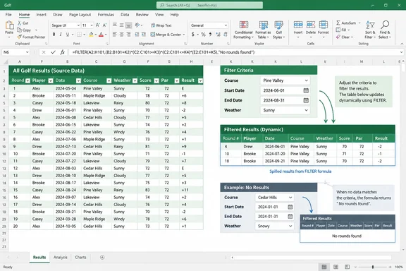
How-To Geek’s September 22 walkthrough demonstrates the technique with a golf-results table, progressively adding course, date, and weather criteria. Microsoft’s FILTER documentation confirms the underlying mechanics, including the use of multiplication for AND conditions and addition for OR conditions. This is an established Excel workflow, not a newly released feature; Geeky Gadgets also described using FILTER with a dynamic selection list in its February 2025 guide.
The useful lesson goes beyond learning another function. A well-built live list separates source records, selection criteria, and results, making a recurring task easier to operate and inspect. Getting that separation right requires attention to table references, output space, and one easily overlooked detail: a “No rounds found” message is still a result cell, which can mislead a downstream count.
Excel FILTER answers a different question from AutoFilter
Excel’s familiar filter arrows are appropriate when you want to inspect a subset of the records already in front of you. Microsoft documents AutoFilter as a way to find, show, or hide values in one or more columns. When records fail the selected criteria, entire worksheet rows are hidden.
That is convenient for a temporary inspection. Select the data, choose Data > Filter, open a column’s arrow, and select or search for the values you want. The result remains in its original location, with nonmatching rows hidden from view.
FILTER instead returns matching values into another part of the workbook. The source stays where it is, and the output occupies its own cells. You can change the selection without repeatedly opening column menus or clearing the source’s filters afterward.
The distinction is particularly useful when your worksheet needs both the complete record set and an answer to a recurring question. In the golf example, the source contains all recorded rounds, while the result answers something narrower: “Show rounds at this course, during this period, in either of these weather conditions.”
| Requirement | Better starting point |
|---|---|
| Temporarily inspect selected rows in an existing table. | Use AutoFilter. |
| Keep the complete source visible while displaying matching records separately. | Use FILTER. |
| Reuse the same selection rules with different input values. | Use FILTER with criteria cells. |
| Edit individual source records after locating them. | Work in the source table; the FILTER output is formula-generated. |
| Produce a result whose size changes as the criteria change. | Use FILTER and leave room for its spilled output. |
Neither method replaces the other. AutoFilter remains a direct way to narrow a working view; FILTER earns its place when the filtered answer becomes a reusable component of the workbook.
An Excel table gives the live list a dependable source
Microsoft lists FILTER for Excel for Microsoft 365, Excel 2024, and Excel 2021, including the corresponding Mac editions, as well as its listed iPad, iPhone, and Android apps. The Windows desktop setup below uses the documented table commands for that environment. Do not infer FILTER availability from the fact that an older Excel version supports ordinary tables or AutoFilter: those are separate capabilities.
The function has three arguments:
=FILTER(array,include,[if_empty])
The array is what Excel should return. The include argument is a corresponding set of TRUE/FALSE decisions identifying which records qualify. The optional if_empty argument tells Excel what to display when none qualify.
A fixed source reference, such as A2:D101, describes a specific rectangle. An Excel table gives the formula a named, expandable source instead. Microsoft documents that structured references—references using table and column names—adjust as data is added to or removed from the table.
That creates two parts of the live-list behavior. The table reference keeps the formula pointed at the current source records, while FILTER determines which of those records belong in the result. Using FILTER against a fixed range does not, by itself, make that fixed range include records added beyond its boundary.
Prepare GolfData before writing the formula
For the example below, the source table needs columns named Course, Date, and Weather, together with whatever other fields you want returned. Those names matter because the formulas refer to them directly. If your workbook uses different names, substitute those exact table and column names rather than copying GolfData[Course] unchanged.
To set up an existing rectangular dataset in Windows Excel:
- Select a cell within the source data and press
Ctrl+T. - Confirm that the selected range contains the intended records and headings. Select My table has headers when the first row contains your field names, then choose OK.
- Select a cell in the new table to expose the Table Design tab.
- Enter
GolfDatain the Table Name box and press Enter. - Reserve an ordinary worksheet area outside the table for the criteria and results.
Microsoft documents both the Ctrl+T creation method and the Table Design naming control. A workbook cannot contain two tables with the same name, so an existing GolfData name must either identify the intended table or be replaced with a different name throughout these examples.
For a clean layout, put the source table on one worksheet and the report area on another worksheet in the same workbook. That is a layout choice rather than a FILTER requirement, but it keeps a growing output from colliding with the source. The formulas below use the table name, so the source does not need to sit beside the result.
Use these report cells consistently:
| Report cell | Purpose |
|---|---|
F2 | The selected course. |
G2 | The inclusive start date. |
H2 | The inclusive end date. |
I2 | The first selected weather category. |
J2 | An optional second weather category. |
F5 | The cell containing the FILTER formula. |
The entire returned table will extend rightward and downward from F5, so this arrangement assumes that area is available. Also, the plain GolfData reference returns the table’s data rows, not its header or totals row. If the report needs headings, place matching headings above the output, outside its spill area.
FILTER turns one criteria cell into a reusable report
Start with only the course condition. Enter a course name that exists in the source’s Course column into F2, then enter this formula in F5:
=FILTER(GolfData,GolfData[Course]=F2,"No rounds found")
GolfData tells Excel to return the source table’s data columns. GolfData[Course]=F2 compares each record’s course with the selected value. "No rounds found" supplies a readable result when no record satisfies that comparison.
How-To Geek uses a data-validation drop-down in F2, but the formula does not require one. A typed value works because FILTER reads the value in the cell, not the control used to enter it. A drop-down is a useful interface refinement; it should not become a prerequisite for understanding or verifying the formula.
Press Enter once. Excel places the matching records in neighboring cells, a behavior Microsoft calls spilling. You do not need to copy the formula down enough rows to accommodate the expected answer.
Check the single-condition result before adding more rules
A gradual build makes mistakes easier to isolate. With only the course criterion active, you can compare the output directly with the source without also reasoning about dates and weather.
- Set
F2to a course you know appears inGolfData. - Confirm that the returned records all have that course value.
- Change
F2to another course present in the table and confirm that the result changes. - Enter a course value absent from the table and confirm that
No rounds foundappears. - Restore the intended course before adding more criteria.
These checks follow directly from the formula’s defined behavior. They establish that the table name, column name, criteria reference, and no-match branch work before the inclusion expression becomes longer.
Only the top-left cell, F5, contains the editable spilled-array formula. Microsoft explains that selecting another cell in the output shows the formula as ghosted text in the formula bar; those generated cells cannot be changed individually. To change the report’s rule, edit F5. To correct a recorded round, edit the source table.
This gives the workbook a clear division of responsibilities. The source holds the records, F2 holds the current selection, and F5 holds the rule that produces the answer. Treating the result as another manually editable table would undermine that arrangement.
AND and OR make FILTER criteria precise
Once the course-only list works, add the date boundaries. Put the start date in G2 and the end date in H2, using date values suitable for comparison with the source’s Date column. Replace the formula in F5 with:
=FILTER(
    GolfData,
    (GolfData[Course]=F2)*
    (GolfData[Date]>=G2)*
    (GolfData[Date]<=H2),
    "No rounds found"
)
Microsoft’s FILTER examples use multiplication to combine conditions with AND logic. In this formula, a record must pass all three tests: the course matches, the date is on or after the start, and the date is on or before the end.
The boundaries are inclusive because the operators are >= and <=. This example assumes that the source’s Date field and the criteria cells represent comparable dates. FILTER applies the comparisons you write; it does not validate the meaning of an imported date field or repair inconsistent source values.
A simple consequence is worth recognizing before troubleshooting: if the start date is later than the end date, no ordinary date can satisfy both boundaries. A no-match result in that situation is consistent with the rule, rather than evidence that the function has stopped working.
Add one weather requirement with another multiplication
To require a particular weather category as well, place that category in I2 and extend the inclusion expression:
=FILTER(
    GolfData,
    (GolfData[Course]=F2)*
    (GolfData[Date]>=G2)*
    (GolfData[Date]<=H2)*
    (GolfData[Weather]=I2),
    "No rounds found"
)
The new weather comparison has the same status as the existing conditions: every returned record must pass it. You have changed the selection rule without changing the source, the result location, or the way the course and dates are entered.
One useful verification follows from that logic. Keeping the course and dates unchanged while adding a mandatory weather condition can only preserve or reduce the qualifying set. If your intended change appears to broaden the selection, inspect the expression and criteria rather than assuming that more conditions always mean a narrower result.
Notice that blank criteria cells are not defined as “All” in these formulas. Each cell participates in an explicit comparison. If you want an optional condition, that would require additional logic; leaving a selector empty does not implement it automatically.
Group alternative weather conditions before combining them with AND
Now suppose either of two weather categories is acceptable. Put the first in I2 and the second in J2, then use addition inside a grouped weather expression:
=FILTER(
    GolfData,
    (GolfData[Course]=F2)*
    (GolfData[Date]>=G2)*
    (GolfData[Date]<=H2)*
    ((GolfData[Weather]=I2)+(GolfData[Weather]=J2)),
    "No rounds found"
)
Microsoft documents addition in FILTER conditions as OR logic. Here, the weather test passes if the record matches either selected category. The course and date requirements remain mandatory.
The parentheses around the two weather comparisons carry the meaning of the rule. Read the expression as “the selected course AND the selected date interval AND either selected weather category.” Adding an ungrouped alternative to the end of a longer expression can describe a different selection than the one you intended.
Selecting the same weather category in both cells does not ask FILTER to return the record twice. The expression still supplies one inclusion decision per source row. This is a consequence of the function’s row-selection mechanism: OR broadens which records qualify; it does not append another copy of each matching record.
The line breaks in these examples are for readability. How-To Geek notes that Alt+Enter can insert a line break while entering a formula. Keeping each test on its own line makes a long expression easier to inspect without changing its logic.
Spill space and empty results determine whether the report stays reliable
A FILTER formula must sit outside an Excel table. Microsoft explicitly states that spilled-array formulas are unsupported inside tables themselves, even though tables are useful sources for those formulas. Put the records in the table and the spilled formula in ordinary worksheet cells.
The output also needs enough available space. Because this example returns every data column in GolfData, its result may grow horizontally as well as vertically when the source structure or number of matches changes. An area large enough for today’s selection may be too small for tomorrow’s broader selection.
Microsoft documents #SPILL! when something blocks the required output range. Selecting the formula cell helps reveal the intended spill area. Before removing anything, inspect whether the obstructing cells contain information you need; moving the report to a clear area is preferable to deleting unrelated work just to make the formula fit.
A practical recovery sequence is:
- Select the cell containing the
#SPILL!error. - Inspect the intended output area and confirm that the formula is outside any Excel table.
- Identify existing content that overlaps the intended result.
- Preserve needed content by moving it elsewhere, or relocate the FILTER formula to a sufficiently clear area.
- Confirm that the matching records now appear, then try a broader selection to assess the space available for growth.
Microsoft’s spilled-array guidance confirms that removing an output blockage allows the formula to spill normally. The important precaution is to treat the obstruction as existing workbook content, not disposable clutter.
“No rounds found” prevents an error but changes the result’s shape
The third argument is optional in the syntax, but it is valuable in an interactive report. Microsoft says FILTER cannot return an empty array; without an if_empty value, a no-match outcome produces #CALC!.
Using "No rounds found" makes that state understandable. Using "" is another documented option, producing an empty string instead. Neither choice creates a genuine zero-row result.
That matters for the count suggested in How-To Geek’s walkthrough:
=ROWS(F5#)
The # spill-range operator refers to the complete current output beginning at F5. When FILTER returns matching records, ROWS counts the result’s rows, so the formula provides the expected record count for this example.
When FILTER returns No rounds found, however, ROWS(F5#) returns 1. It is counting the single row occupied by the fallback message. An empty-string fallback does not turn that output into a zero-row range either.
The safe interpretation is therefore narrower than “number of matching records in every state.” This formula counts the rows of the spill. If you use it as a report metric, its label or surrounding logic must account for the no-match branch; otherwise the report can display a message saying there are no records beside a count saying there is one.
A no-match fallback does not handle every error
if_empty handles an absence of matching records. It is not a general-purpose error handler. Microsoft warns that FILTER returns an error if the inclusion array contains an error or a value that cannot be converted to a Boolean decision.
If a previously working report begins failing, inspect the source values used by the conditions as well as the output area. A comparison involving an erroneous source cell is a different problem from a legitimate set of criteria that matches nothing.
Workbook boundaries introduce another documented limit. Microsoft supports dynamic-array links between workbooks only when both workbooks are open; closing the source workbook can produce #REF! when the linked formula refreshes. Keeping the source and report on separate worksheets within the same workbook avoids introducing that particular cross-workbook dependency.
Sorting is a reasonable next extension once these basics work. Microsoft demonstrates nesting FILTER inside SORT to order the returned records. That should remain a separate design choice from selection: first establish which records belong in the report, then choose the field and direction that determine their order.
Build one dependable FILTER view before expanding the workbook
Start with a recurring selection task that already has a clear source table and a small number of criteria. Establish a correct one-condition report, exercise its no-match behavior, and then add the extra conditions you actually use. There is little benefit in constructing an elaborate dashboard before confirming that its simplest result is dependable.
For shared workbooks, the main checks are practical rather than cosmetic. Confirm that recipients use a FILTER-capable Excel version, keep the source and output roles obvious, and avoid presenting a spill-row count as an unconditional record count. These are the details that determine whether another person can rely on the workbook without understanding every part of its formula.
- Use AutoFilter for a temporary narrowed view, and use FILTER when you need a separate result that changes with criteria cells.
- Put expanding source data in an Excel table and reference its table and column names so added records remain within the formula’s source.
- Enter the FILTER formula outside the table and reserve clear space for the largest result you expect to display.
- Multiply conditions that must all hold, and group alternative conditions joined with addition before combining them with the mandatory tests.
- Verify the no-match state, including any downstream counts, and keep both workbooks open if the report depends on a dynamic-array link to an external source.
The durable improvement is a workbook with an explicit, reusable selection rule. Once the course-only example works, the date and weather requirements become understandable extensions of the same formula rather than another sequence of filter-menu clicks. Keep AutoFilter for inspecting the source; use FILTER when the answer deserves a stable place of its own.
References
- I stopped overrelying on Excel's filter buttons after learning how to build live lists How-To Geek · 2026-09-22T11:00:13+00:00
- FILTER function | Microsoft Support support.microsoft.com