

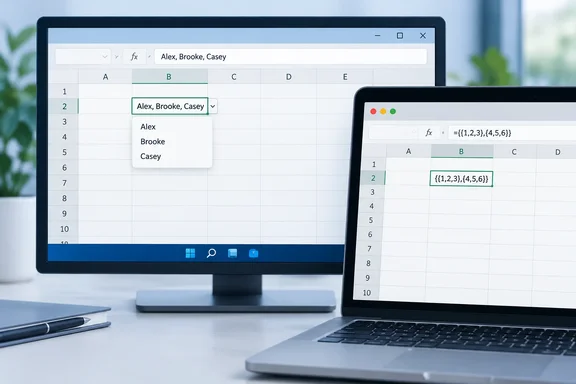
Excel lists put "Carlos, Henrietta, Jacob" back into one cell
Microsoft's Microsoft 365 Insider blog announced the change on September 24, 2026. It starts from something every spreadsheet user has seen: many workbooks already try to pack multiple values into one cell. A project might list "Carlos, Henrietta, Jacob" as three owners, or a Forms survey might return "2:00 PM; 2:30 PM; 3:00 PM" as one response. Until now, Excel treated each of those as one text string. You could split it apart with a formula, but you couldn't filter on "Henrietta" without a wildcard text match.
A list keeps the look of that packed cell but changes how Excel reads it. According to Microsoft, with lists, you can keep those values in one cell, while also keeping them separate for filtering, calculation and more. The cell stays compact, and Excel knows where each item starts and ends.
The Excel team published a companion post on the Excel Blog that takes the same idea further, into project data. Its example is a website launch with separate design, development, and testing workstreams, each with its own milestones. The Excel team says nested arrays help preserve those relationships, keeping milestone groups tied to the workstream they belong to rather than combining everything into a single list.
People outside Microsoft have already shown the feature working. Excel MVPs Mynda Treacy of MyOnlineTrainingHub and Leila Gharani both posted YouTube walkthroughs recorded on Beta builds, and summaries of those videos describe the same Ctrl+J workflow and new functions that Microsoft documents. A summary of Treacy's video notes that the recording comes from the Microsoft 365 Beta Channel preview, so the features shown may not yet be available to all users.
How to create, edit, and filter a list in Excel Beta
Creating a list is the easy part of the announcement, and it is the part most Beta users will try first. Microsoft documents these steps:
- Select a cell and choose Insert > List, or press Ctrl+J.
- Type or paste the items, separated by commas or semicolons. Which separator works depends on your Windows or macOS regional settings.
- Select the icon that appears in the cell to see the individual values.
- To add, remove, or change items later, double-click the cell or press F2, the same way you edit any other value.
If it worked, the cell shows the list icon and the items appear separately when you open it. The regional-settings detail is worth noticing. In locales that use a comma as the decimal separator, Excel normally uses semicolons as its list separator, so pasting comma-separated data may not split the way a US user would expect.
Filtering gets better straight away. Microsoft says you can filter by one or more individual items instead of whole text entries. On a project tracker, that means filtering the Owners column to "Jacob" returns every project Jacob is on, even when he shares the cell with two other people.
Lists also work in formulas. Referencing a list returns all its values, and Microsoft's example is =B2, which spills the items into separate cells. So a plain cell reference to a list does not stay in one cell. It expands into the grid the same way a dynamic array does. The Gharani video summary says existing functions like COUNTA, SUM, SORT, and XLOOKUP adapt to work with these lists automatically. That comes from an MVP demonstration, not a Microsoft compatibility list, so check it against your own formulas.
Braces in Excel formulas now keep a spilled array inside one cell
Lists are the simple case of a deeper change. Microsoft says that for the first time in Excel, arrays can exist natively in cells as values or as formula results. They can be any size or shape, and they can contain other arrays.
Here is how it works. Since dynamic arrays arrived, a formula like ={1;2;3} has spilled its three results down three cells. Excel has always used braces to write array constants. The new rule allows more than one layer of them. By Microsoft's description, wrapping the original array in braces creates a 1??1 array around it, so the result stays in one cell instead of spilling. Applying that rule, ={{1;2;3}} gives one cell holding a three-item array.
Microsoft says the same wrapping works on the body of any spilling formula, not only on constants. The practical benefit is layout. You no longer have to leave empty cells below or beside a formula for its spill, and you won't hit a #SPILL! error because something is already in the way. The array sits in its cell until another formula uses it.
That makes table designs possible that weren't practical before. Microsoft's example is a running tracker with one run per table row. The kilometer split times for each run are stored together, even though a 5K and a half marathon have different numbers of splits, and each run's statistics are calculated in the same row. Before this, the usual approaches were a separate splits table joined by a run ID, or a ragged block of columns sized for the longest run.
Nested arrays end the #CALC! wall for TEXTSPLIT and friends
Advanced formula writers have been waiting for this part. Arrays can now nest inside other arrays, as in ={{1,2,3};{4,5,6}}. Microsoft says a formula that produced an array of arrays used to return a truncated result or a #CALC! error. Now supported formulas return the complete nested result.
Microsoft demonstrates the fix with TEXTSPLIT. Applied row by row to a column of delimited text, the old behavior returned only the first item for each row. With nested arrays, the result spills one array per row, and each row's array can be used in further calculations. Anyone who has written a BYROW and TEXTSPLIT combination and hit #CALC! has seen this limit.
Note Microsoft's wording: supported formulas return the complete nested result. The announcement does not promise that every function understands nested input. The Treacy video summary says her demo covered nested-array math using LET, MAP, and LAMBDA to compute totals from lists inside cells, which suggests the LAMBDA helper functions are among the ones that work.
FLATTEN, HAS, HASANY and HASALL are Excel's new array functions
Microsoft added four functions for working with this data:
| Function | Syntax | What it returns |
|---|---|---|
| FLATTEN | FLATTEN(array, [pad_value], [levels]) | The array with one or more levels of nesting removed, spilled into the grid |
| HAS | HAS(array, value) | TRUE if the value appears anywhere in the array, otherwise FALSE |
| HASANY | HASANY(array, values) | TRUE if any of the values appear anywhere in the array, otherwise FALSE |
| HASALL | HASALL(array, values) | TRUE if all of the values appear anywhere in the array, otherwise FALSE |
FLATTEN(array, [pad_value], [levels]) simplifies nested arrays by removing one or more levels of nesting. Continuing from the prior example, FLATTEN lets you simplify the nested array output, spilling the individual results into the grid. The pad_value argument handles ragged data. In Microsoft's TEXTSPLIT example, an empty string ("") as the pad value makes rows with fewer items show blanks in the remaining columns. Without it, you'd expect the usual error fill for missing positions. The levels argument sets how many layers are removed, which only matters once arrays are nested more than one deep.
The three HAS functions are membership tests, and they fit the project-tracker case closely. The Excel Blog frames them this way: HAS finds projects owned by a specific person, HASANY finds projects that involve any member of a leadership team, and HASALL finds projects that include every required stakeholder before launch? Use HASALL. Before this, a check like that took ISNUMBER(SEARCH()) wrappers over text, which break when one name is contained in another.
Microsoft counts four new functions. Some third-party video summaries group the existing GROUPBY function with them and mention "five". GROUPBY and PIVOTBY show up in the MVP demos as tools for summarizing list data, but they are not part of this announcement.
Compatibility Version 3 is the switch that turns nested arrays on
This is the part that matters most for anyone who shares workbooks. Microsoft says Compatibility Version 3 will be released alongside arrays in cells and is required for most calculations involving nested arrays. You can set Compatibility Version for each workbook in by selecting Formula > Calculation Options. Microsoft's support documentation gives the full path as Formulas > Calculation Options > Compatibility Version.
Compatibility Versions are a per-workbook setting that Microsoft introduced so function behavior can change without silently breaking old files. Workbooks created before the feature are treated as Version 1. Version 2 changed LEN, MID, FIND, SEARCH, and REPLACE to count Unicode surrogate pairs, such as most emoji, as one character. Microsoft's support page, as of this writing, still lists Version 2 as the highest available version in every channel, Beta included. It doesn't document Version 3 yet, so the Insider post is the only official description of it for now.
The warning comes with it: some existing formulas return different results in Compatibility Version 3. If your workbook doesn't behave as expected, you can keep it set to Compatibility Version 1 or 2. Microsoft doesn't say which formulas change. A likely inference, not something Microsoft has confirmed, is that formulas which used to return #CALC! or truncate nested results will now return full nested arrays, and that can ripple into the cells that depend on them. Until Microsoft publishes the list, compare results before and after you switch a workbook.
Six Excel features that don't understand arrays yet
Microsoft lists six known limitations in the Beta release. They decide whether lists fit into an existing reporting workflow:
- Conditional formatting doesn't inspect array contents unless you use a formula-based rule.
- Data validation can't use a list or array as the source for dropdown items.
- Charts don't expand an array into separate data points.
- PivotTables don't read array values as source data.
- Power Query doesn't load or emit array-valued columns.
- Find & Replace can't replace individual list or array items.
Together these cover most of the ways workbooks are consumed downstream. If a tracker feeds a PivotTable, a chart, or a Power Query refresh, turning its owner column into lists would break those links today. The Treacy walkthrough reaches the same conclusion, noting that integration gaps remain (for example, with PivotTables and Power Query). The workaround available now is to FLATTEN array data into ordinary cells before a PivotTable or chart reads it. Microsoft's FLATTEN description supports that, though Microsoft doesn't present it as an official workaround.
What this means for you
If you're on the Beta Channel and like to experiment, try lists in a throwaway copy now. Everyone else, including anyone who manages Excel for other people, should wait for general availability. The rollout builds are Version 2610 (Build 20520.20000) or later on Windows and Version 16.114 (Build 26092111) or later on Mac. Even on those builds, Microsoft says features covered on this blog roll out over time to enable us to monitor quality and performance, so some preview features may not be available to you right away. Microsoft also says features can be paused, adjusted, or removed during the rollout, so a workbook built around them in Beta could stop working later.
The announcement covers Excel for Windows and Mac Beta only. It says nothing about Excel for the web, iOS, Android, or the Current and Enterprise channels. Wider availability, and how older builds will open workbooks that contain lists, are open questions until Microsoft publishes more.
- Test lists and nested arrays only in copies of workbooks. Microsoft explicitly advises against using them in important files before general availability.
- Check your build against Version 2610 (Build 20520.20000) on Windows or 16.114 (Build 26092111) on Mac, and expect a staged rollout even on qualifying builds.
- Keep production workbooks on Compatibility Version 1 or 2, because Microsoft says some existing formulas return different results under Version 3.
- Don't convert columns that feed PivotTables, charts, Power Query, or data-validation dropdowns, since none of them read array values in the preview.
- Try HAS, HASANY, and HASALL wherever you now use ISNUMBER(SEARCH()) text matching on delimited names or tags.
- Send feedback through Help > Feedback in Excel. Microsoft says the behavior may change based on it before release.
Lists and nested arrays are the biggest change to Excel's data model since dynamic arrays. The Ctrl+J list solves a problem every Forms export and project tracker already has, and nested arrays fix the #CALC! limit that has held back advanced formulas. Before this reaches most users, two things need to happen: the six integration gaps have to close, and Compatibility Version 3 has to appear in Microsoft's formal documentation with a list of the formulas it changes. Until then, stick with conventional tables for anything that feeds reports, and use a spare copy to see how your own workbooks would change.