Excel: 5 Built-In Tools to Navigate, Audit and Compare Workbooks

A productive Excel weekend does not require learning a new formula language or rebuilding every workbook from scratch. Five underused tools already built into Excel can cut down on repetitive scrolling, messy imports, manual auditing, and constant tab-switching—provided users understand where each feature excels and where it can create trouble.
For Windows users who spend Monday mornings cleaning up exported reports, reconciling numbers, or trying to locate one stubborn formula in a vast worksheet, these are practical skills worth testing in a low-pressure session. The payoff is not merely a faster spreadsheet; it is a workflow that is easier to review, less error-prone, and far more manageable when data grows beyond a few hundred rows.

---

Overview: Small Excel Habits, Significant Time Savings​

Excel productivity is often framed around advanced functions, Power Query transformations, macros, or elaborate dashboards. Those tools matter, but the biggest time savings frequently come from simpler actions repeated dozens of times per day.
Consider the routine friction points in a typical workbook:

• Scrolling endlessly to reach a distant cell
• Pasting external data and repairing its formatting afterward
• Hunting through columns to distinguish formulas from manually entered values
• Trying to compare summary figures with raw data on another sheet
• Receiving an unfamiliar workbook and needing a quick sense of what the numbers reveal

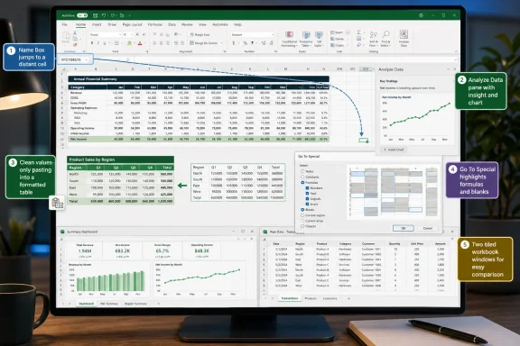
The five features below address those exact problems:

1. The Name Box for direct workbook navigation and range selection
2. Analyze Data for automatic summaries, charts, and natural-language questions
3. Paste Values with Ctrl+Shift+V for cleaner data imports
4. Go To Special for auditing formulas, constants, blanks, and validation rules
5. New Window and Arrange All for viewing different areas of one workbook simultaneously

None of these capabilities is a replacement for good spreadsheet structure. A workbook with inconsistent headers, merged cells, hidden logic, and unexplained calculations will still be difficult to maintain. But each feature can reduce the time spent navigating that complexity.

Use the Name Box to Navigate Large Workbooks​

The Name Box is one of Excel’s most overlooked navigation tools. It sits at the left edge of the formula bar and normally displays the address of the active cell, such as B14 or H207.
Most people treat it as a passive display. In reality, it is an efficient command field for moving around a worksheet and selecting ranges without touching a scroll bar.

Jump Directly to a Cell​

Click the Name Box, type a cell reference, and press Enter.
For example:

• Type A650 to move directly to cell A650
• Type XFD1 to jump to Excel’s farthest possible column and first row
• Type M25000 to inspect a record deep inside a large data set

This is especially useful in workbooks containing exports from accounting systems, CRM platforms, inventory tools, or web analytics platforms. Dragging the vertical scroll bar through tens of thousands of rows is slow, imprecise, and frequently leads to overshooting the intended location.
The Name Box offers a much cleaner alternative. Instead of navigating visually, users navigate by reference.

Select a Complete Range Instantly​

The Name Box also selects a range when given a range reference.
Typing D2:J100 and pressing Enter highlights every cell in that block. That makes it useful for tasks such as:

• Applying a number format to a defined section
• Creating a chart from a known block of data
• Clearing only a designated input range
• Copying a report segment without dragging through it
• Checking whether a formula was filled down consistently

For non-adjacent selections, the Go To dialog remains more flexible. But for a single rectangular range, the Name Box is faster than dragging across a crowded worksheet.

Turn Important Areas into Named Ranges​

The Name Box becomes even more useful when it is used to create named ranges. Select a cell or range, click the Name Box, type a descriptive name, and press Enter.
A range might be named:

• MonthlySales
• InputArea
• TaxRates
• DashboardKPIs
• NorthRegionData

Once defined, the name appears in the Name Box drop-down list. Clicking it returns the user to that range immediately.
This is a simple way to make a workbook more navigable, particularly when it contains several worksheets and a mixture of input areas, calculations, summary tables, and reference lists. A named range can also make formulas more readable. A formula such as =SUM(MonthlySales) is easier to interpret than =SUM(F2:F1500).

The Limits of the Name Box​

The Name Box is deceptively simple, but it is not a complete workbook-management system. Names can be workbook-level or worksheet-level, and poorly managed names can become confusing in heavily edited files.
Users should avoid vague or temporary names such as Data1, Range2, or Test. Descriptive names are more durable. It is also important to remember that naming a range does not protect it, validate its contents, or document its business purpose.
For more complicated situations—such as names with broken references, sheet-specific scope, or formulas that dynamically expand—Excel’s Name Manager is the better review tool.
Still, as a daily navigation shortcut, the Name Box deserves a place in every Excel user’s muscle memory.

---

Let Analyze Data Find Patterns Before Building a Report​

Excel’s Analyze Data feature is designed for a familiar situation: a worksheet contains plenty of numbers, but no immediate explanation of what matters.
Instead of building a PivotTable, selecting fields, testing chart types, and experimenting with filters from scratch, Analyze Data examines a selected data range and suggests summaries, trends, tables, and visualizations. It can also respond to natural-language prompts.

How Analyze Data Works​

Click inside a structured data set and select Home > Analyze Data. Excel opens a task pane that proposes relevant views of the data.
Depending on the contents of the sheet, it may suggest:

• Totals and averages
• High and low values
• Category comparisons
• Time-based trends
• PivotTable-style summaries
• Charts based on key fields
• Distribution views for numerical columns

Users can insert a suggested output directly into the worksheet. That can be a useful starting point for a quick report, an exploratory analysis, or a management update that needs basic context before deeper work begins.

Ask Questions in Plain English​

The feature becomes more valuable when users know the question they want answered but do not want to build the report manually.
Useful prompts can include:

• “Total sales by region”
• “Average cost by month”
• “Which product has the highest profit?”
• “Show revenue by quarter”
• “Top five customers by order value”
• “Count orders by status”

This approach can reduce the barrier to analyzing an unfamiliar data set. A user inheriting a workbook does not necessarily know which fields belong in a PivotTable or whether dates are stored consistently enough for grouping. Analyze Data can surface possible relationships more quickly than a manual first pass.

Why It Is Helpful—but Not a Replacement for Judgment​

The major strength of Analyze Data is speed. It is an effective way to create an initial view of a clean, tabular data set.
Its limitation is equally important: Excel can summarize data, but it cannot determine whether the data is meaningful, complete, properly categorized, or appropriate for the question being asked.
A chart may look persuasive while hiding major issues:

• Duplicate records may inflate totals
• Text-formatted dates may prevent accurate grouping
• Empty values may be treated differently than zeros
• Categories may have inconsistent spellings
• An unusual outlier may distort averages
• A column labeled “Revenue” may actually contain gross sales rather than net sales

Analyze Data should therefore be treated as an exploratory tool, not a final authority. Its suggestions can reveal patterns worth investigating, but they should not be inserted into a decision-making report without validation.

Availability and Compatibility Considerations​

Analyze Data is primarily tied to Microsoft 365 desktop subscriptions and may vary by update channel, language, region, and organizational settings. Some users may still see the feature under its earlier name, Ideas.
Natural-language querying can also be inconsistent if headers are unclear or the underlying range is poorly structured. The better the column names and the cleaner the table, the more useful the results will be.
For best results:

1. Use one header row only.
2. Avoid merged cells in the data range.
3. Ensure each column contains one type of information.
4. Remove entirely blank rows inside the data.
5. Convert the range to an Excel Table where appropriate.
6. Check that dates and numbers are stored as real dates and numbers.

Analyze Data is not magic. It is most effective when the worksheet already follows the basics of good data design.

---

Use Ctrl+Shift+V to Paste Values Without the Formatting Chaos​

Copying and pasting is one of the most common Excel actions, and it is also one of the easiest ways to damage a workbook’s consistency.
A standard Ctrl+V paste can bring across more than visible values. Depending on the source, it may include:

• Fonts and font sizes
• Fill colors
• Borders
• Number formats
• Formulas
• Hyperlinks
• Data validation
• Comments or notes
• Conditional formatting
• Column widths

That behavior is sometimes necessary. Often, it is exactly what users do not want.

The Fast Paste-Values Shortcut​

In newer versions of Excel for Microsoft 365, Ctrl+Shift+V can paste values while retaining the destination formatting. This is ideal when copying data from another workbook, an email, a web page, or a calculation sheet into a clean reporting template.
The result is straightforward:

• The destination sheet keeps its own fonts, fills, and borders.
• Formulas copied from a source range are converted to their displayed results.
• Existing formatting in the receiving cells remains intact.

For example, if a polished financial-report template uses a particular date format, currency format, font, and shading scheme, paste values prevents an imported range from overwriting that design.

Practical Uses for Paste Values​

This shortcut is useful in everyday scenarios:

• Bringing exported text from a web portal into a prepared table
• Copying calculated results into a permanent snapshot
• Moving data from an external workbook without importing formulas
• Replacing formulas with their current results before sharing a file
• Inserting copied names or lists without inheriting strange fonts and spacing
• Avoiding inconsistent colors after pasting from email or browser content

It is also a practical defense against accidental external links. Standard copying between workbooks can sometimes preserve formulas or references that users did not intend to bring along. Pasting values helps ensure that the destination receives the visible result rather than the logic behind it.

A Critical Compatibility Warning​

The Ctrl+Shift+V shortcut is not equally available in every version, build, or edition of Excel. Older perpetual-license versions may not support it in the same way, and some users may encounter different paste behavior based on their installed Microsoft 365 update channel.
That distinction matters in shared offices. A shortcut that works perfectly on one Windows PC may not work for a colleague using an older Excel release.
The broadly compatible fallback remains:

1. Copy the source data with Ctrl+C.
2. Select the destination cell.
3. Press Ctrl+Alt+V to open Paste Special.
4. Choose Values.
5. Confirm the action.

It is not as fast, but it is dependable and gives users more control over exactly what is pasted.

Paste Values Is Not Always the Correct Choice​

Pasting values can be destructive if the formulas themselves are important. A formula such as =SUM(B2:B20) becomes a fixed number after a values-only paste. That may be useful when preserving a historical snapshot, but it removes automatic updates.
Use values-only pasting when the destination should contain a static result. Use normal paste or formula paste when the destination workbook needs live calculations.
This is a subtle but essential distinction. Speed is valuable, but preserving the intended behavior of the workbook is more important.

---

Use Go To Special to Audit a Worksheet in Seconds​

Go To Special is one of Excel’s most powerful built-in auditing tools. It enables users to select cells based on their type or characteristics rather than their visible location.
Instead of visually scanning a large worksheet to find formulas, hard-coded entries, blanks, validation rules, or cells with conditional formatting, users can ask Excel to select every matching cell at once.

Opening Go To Special​

There are several ways to reach it:

• Press F5, then select Special
• Press Ctrl+G, then select Special
• Choose Home > Find & Select > Go To Special

Before opening the command, decide whether the task applies to the full worksheet or only a specific area.

• Select a single cell to inspect the entire worksheet.
• Select a range first to limit the search to that region.

This small decision matters. Auditing an entire worksheet can be useful, but it can also select more cells than expected in a workbook with numerous support areas, hidden calculations, or imported data.

Find Every Formula​

Choosing Formulas selects cells that contain formulas. This is particularly useful when inheriting a workbook and trying to understand where calculations actually occur.
Once selected, formulas can be:

• Highlighted with a temporary fill color
• Reviewed with the Formula Bar
• Added to the Watch Window
• Checked for inconsistent patterns
• Copied into a separate audit sheet
• Protected to prevent accidental changes

It is also useful for spotting a common spreadsheet problem: a column that should contain formulas all the way down but includes a few manually typed values instead.

Find Constants and Hard-Coded Inputs​

Choosing Constants highlights cells containing manually entered values rather than formulas.
This is valuable when reviewing models, budgets, pricing sheets, or planning workbooks. Hard-coded numbers are not automatically errors, but they deserve attention when they appear inside a calculation area.
A simple audit pattern is:

1. Select the calculation region.
2. Run Go To Special > Constants.
3. Apply a temporary fill color.
4. Review whether those entries are intended assumptions or accidental overrides.
5. Remove the temporary formatting after the audit is complete.

This can reveal an old manually entered discount rate, a pasted total that replaced a formula, or a one-off adjustment buried in a column of calculations.

Find Blanks Carefully​

Blanks is useful but risky. It selects empty cells within the chosen range, and users can then fill or format those cells simultaneously.
For example, if a table should have a value in every row of a specific column, selecting blanks can quickly expose missing information. It can also be used to fill gaps with a default value or formula.
However, deleting rows based on selected blanks is dangerous. Real worksheets may contain intentional gaps, section breaks, optional fields, uneven data structures, or partially completed records. A blanket delete can remove valid records or shift related data out of alignment.
A safer approach is to add a helper column that evaluates whether a full record is complete. That makes the deletion rule visible, repeatable, and easier to verify.

Other Useful Options​

Go To Special can also find:

• Cells with data validation
• Cells with conditional formatting
• Visible cells only in filtered lists
• Errors such as #N/A, #VALUE!, or #DIV/0!
• Comments or notes
• The current region
• The last cell used on a worksheet

The visible-cells-only option is especially useful when copying filtered data. Without it, copying a filtered range can include hidden rows in ways that surprise users.

Why Go To Special Matters for Excel Quality Control​

The feature turns visual searching into structural analysis. It does not fix errors automatically, but it makes the workbook’s hidden patterns visible.
That is the key advantage. Large spreadsheets are difficult not because they contain many cells, but because it is difficult to know which cells contain logic, which contain manual assumptions, and which are empty for a reason. Go To Special makes those distinctions easier to inspect.

---

Open a New Window to Compare Different Parts of the Same Workbook​

A second Excel window can eliminate one of the most frustrating parts of spreadsheet work: switching back and forth between distant tabs or rows.
The New Window command does not create a second copy of the workbook. It opens another view of the same workbook, with the same data and the same underlying file.

Set Up a Side-by-Side Comparison​

To create another view:

1. Open the workbook.
2. Select the View tab.
3. Choose New Window.
4. Return to the View tab.
5. Select View Side by Side or Arrange All.
6. Choose the layout that suits the task.

The most useful layouts include:

• Vertical for side-by-side comparisons
• Horizontal for stacked views
• Tiled for viewing several windows at once
• Cascade for quickly switching among overlapping windows

This lets users keep a summary sheet visible in one window while examining source data in another. It also allows a comparison between the beginning and end of a lengthy worksheet without endless scrolling.

Useful Scenarios for Multiple Workbook Views​

New Window is particularly effective for:

• Checking dashboard figures against raw transactions
• Comparing monthly and quarterly summary sheets
• Reviewing formulas in one section while viewing inputs elsewhere
• Comparing two distant areas of the same worksheet
• Matching a lookup table to the output that depends on it
• Reviewing data before and after a transformation
• Monitoring a control total while making adjustments

Edits made in one window appear in the other because both windows point to the same workbook. This is convenient, but it is also a reason to remain cautious.

Use Synchronous Scrolling When It Helps​

When comparing two sheets with the same structure, Synchronous Scrolling can move both windows together. This is ideal for before-and-after comparisons, regional worksheets built from the same template, or duplicated periods such as current-year and prior-year reports.
It is less useful when the sheets are structured differently. In that case, side-by-side viewing without synchronized scrolling gives more control.

Avoid the “Two Copies” Misunderstanding​

A new workbook window is not a backup. Saving changes in either view saves them to the same file. Closing one view does not close the workbook if another view remains open, but closing the final view ends the session normally.
The extra window should therefore be treated as a navigation aid, not a safety mechanism. For risky edits, use version history, a separate backup copy, or a clearly labeled test workbook.

---

Build a Faster Excel Workflow Without Sacrificing Accuracy​

The five tools share a common theme: they reduce movement and repetition.
The Name Box reduces scrolling. Analyze Data reduces the time required to form an initial summary. Paste Values reduces cleanup. Go To Special reduces manual searching. New Window reduces switching between distant areas of a workbook.
Together, they create a more deliberate Excel workflow:

• Navigate directly instead of scrolling blindly.
• Explore data before building a complex report.
• Paste only what the destination sheet needs.
• Audit cell types rather than searching visually.
• Compare sheets and ranges without losing context.

The strongest Excel users are not always the people who know the largest number of formulas. They are the people who can move through complex workbooks confidently, preserve the logic that matters, and spot problems before those problems spread into reports or decisions.
A few minutes spent practicing these built-in Excel features can make routine spreadsheet work faster on Monday—and make the resulting workbook more reliable long after the weekend ends.

---

References​

1. Primary source: How-To Geek
   Published: 2026-07-24T22:00:13+00:00
   
   

   5 time-saving Excel tips to put to the test this weekend (July 24-26)

   Don't waste time navigating, analyzing, cleaning, auditing, and comparing data—Excel can do it in minutes.

   www.howtogeek.com
2. Official source: support.microsoft.com
   
   

   Compare two or more worksheets at the same time | Microsoft Support

   Compare two worksheets in the same or different workbooks by viewing them side by side. You can also arrange multiple worksheets so that you can compare them.

   support.microsoft.com